Shutter, Camera and Histogram Equalization

Shutter, Camera and Histogram Equalization

This post consists of:

1. Explain an idea which can be used in a start-up which uses computer vision. No need to explain the algorithms and how-tos.
2. What is “Shutter Speed” feature in cameras and how it can impact on image quality?
3. Implement the equalize_hist1 and equalize_hist2 functions regarding following steps:
   1. Implement histogram equalization via open_cv in equalize_hist1
   2. Implement histogram equalization based on the what have been taught in slides in equalize_hist2
   3. Plot the T function
   4. Plot the histogram of images before equalization and after it.
   5. Explain the differences

1. Explain an idea which uses computer vision

In this section, I want to talk about the idea so-called Lie detection based on body language. This explanation consists of these parts:

1. Intro
2. Usage
3. Reference

1.1 “Lie Detection Based on Body Language” Introduction

I would like to kick of by mentioning the point that as all of us know, when people attempt to lie (orally), they illustrate some signs on their bodies particularly on their faces or hands. In this report, I will focus on the simplified one which only focuses on children’s hands and faces’ major signs, for instance blinking abnormally to help parents detect the lies and help their children to overcome the hardship without losing the control of circumstances.

1.2 Usage

Based on what I have mentioned in the intro section, we can say a group of signs in most cases can lead to a lie confidently¹. And all of those signs have been extracted by experts like agents in police departments so they are all reliable features. For a simple demonstration, we can say the children who start scratching their noses or the back of their heads at the time of talking to their parents or teachers, mostly they are trying to deceive their contacts.².

This proposal has aimed these facts to create a automated system for parents and teachers to capture images while speaking to the children and detect lies. On top of that, parents or teachers will be able to manage the situation and try to understand why their children or students are trying to lie to them. One of the possible causes of lying by children could be feeling insecure about their own abilities. In this kind of situation, the teacher or parent will notice that using this system and instead of putting more pressure on the child or speaking in the way that may cause more fear, try to conciliate and help children by giving them confidence³.

The scale of capturing can be used in three level:

1. Capturing the whole body and focusing only on prominent body language characteristics
2. Capturing face/hands to explore the possibilities using more detailed features.
3. Capturing eye/lips/shaking and heat level (not considered as body language but very useful) to expand the feature pool.

1.3 References

1. Human Lie Detection and Body Language 101: Your Guide to Reading People’s Nonverbal Behavior - Vanessa Van Edwards
2. How to detect lies body language - Nick Babich on Medium
3. Social and Cognitive Correlates of Children’s Lying Behavior - Victoria Talwar and Kang Lee

2. The Impact of “Shutter Speed” On The Quality of Captured Images via Camera

In this section, questions such as what is shutter speed, what is its impact will be answered in the following sections:

1. Shutter Intro
2. Shutter Speed and Its Effects
   1. Exposure (Brightness)
   2. Motion
3. Final Words
4. References

2.1 Shutter Intro

As we know, cameras take photos by exposing their digital sensors to the light. Shutter, as its name illustrates, is a barrier that keeps the light out from the camera’s sensors and it opens when you try to take photo by pressing shutter button on your camera and closes after the photo has been taken which means after closing, sensors are no longer exposed to the light.

2.2 Shutter Speed

Based on what we read in previous section, camera only take photo when its shutter is open, so now a parameter emerges; the speed. The shutter speed is the time it takes from opening shutter and exposing sensors to the light till closing it and it is categorized into two major types:

1. Fast: Conventionally a small fraction of a second for instance 1/100th second or 1/200th second to 1/4000th second.
2. Slow Conventionally more than a second for instance 1, 5, even 30 or a few minutes depends on the task.

These spectrum of speeds have completely different effect on the taken photo from making it brighter or darker or even blurry or sharp. Having a slow shutter means more exposure to the light and in case of brightness, the sensors would gain more light and vice versa. Meanwhile, if object moves, slow shutter means blurry images and vice versa. These will be discussed in the following section more detailed.

2.2.A Exposure

Let say object and subjects are still and we use slow shutter. In this situation, the sensors have more time to absorb the light and it means we will have brighter images. It is very useful in dark environments specially night scenes. But you need to consider that exposing too much to light means a fully bright image of the scene called overexposed, on the other hand, have a quick shutter in dark environment will give a dark image. But shutter speed is not the only factor that impacts the brightness, others are ISO and Aperture which we do not discuss here.

Below is an image that portrays the effect of the shutter speed on the brightness:

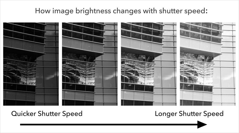Photo: photographylife.com

2.2.B Motion

In this section, the being still constraint has been removed which means the subjects can move at different speeds while the shutter is open (the camera itself can move too but the effect is almost same). It is known to us that the image could be created when light reflects from the objects and if let say point x, exposes to different sensors of camera, its effect will be all there so moving an object while the camera is taking photo means different points of the objects will be reflected on many different sensors not just one and it causes a blurry image as we have seen this effect in rolling shutter or global shutter designs. Actually, it is all about time and because we have a slow shutter, the output will be blurry. Note that if nothing moves, it will not be blurry, only objects that moves create blurry effect in the path they move along and many photographer use these may seem drawback as a upside and create fascinating images that only a part of a image is blurry which is called Motion Blur. Below is the example:

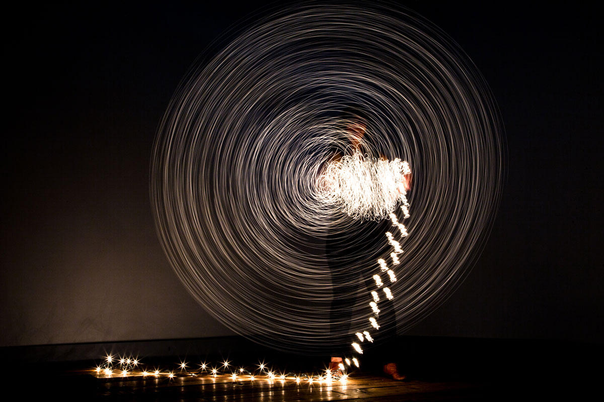Photo: Casey Cosley

On the other hand, if we use a fast shutter, no matter object are moving (but it is important how fast they are) we can achieve a stabilized and still image of the moving object without introducing blur effect. The reason is when shutter closes very fast, each point of the object only reflect on a very small number of sensors and it seems to that objects are stand. One point that will not be waste of time to mention is that if camera and the objects move at the same pace, the image will not be blurry but it is a little bit tricky to acquire. Below is an example of fast shutter on moving object:

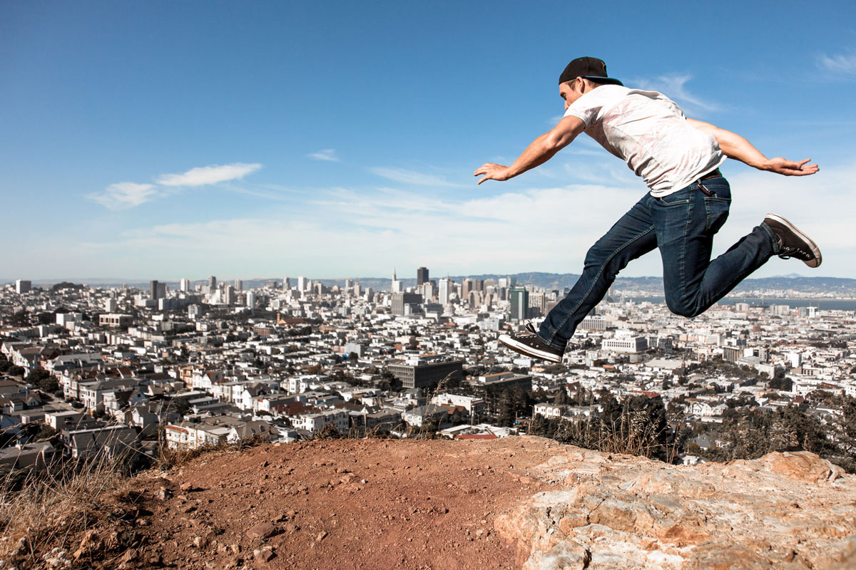Photo: Matt McMonagle

To finish this section, a image that demonstrates the differences between shutter speed and blur effect is great.

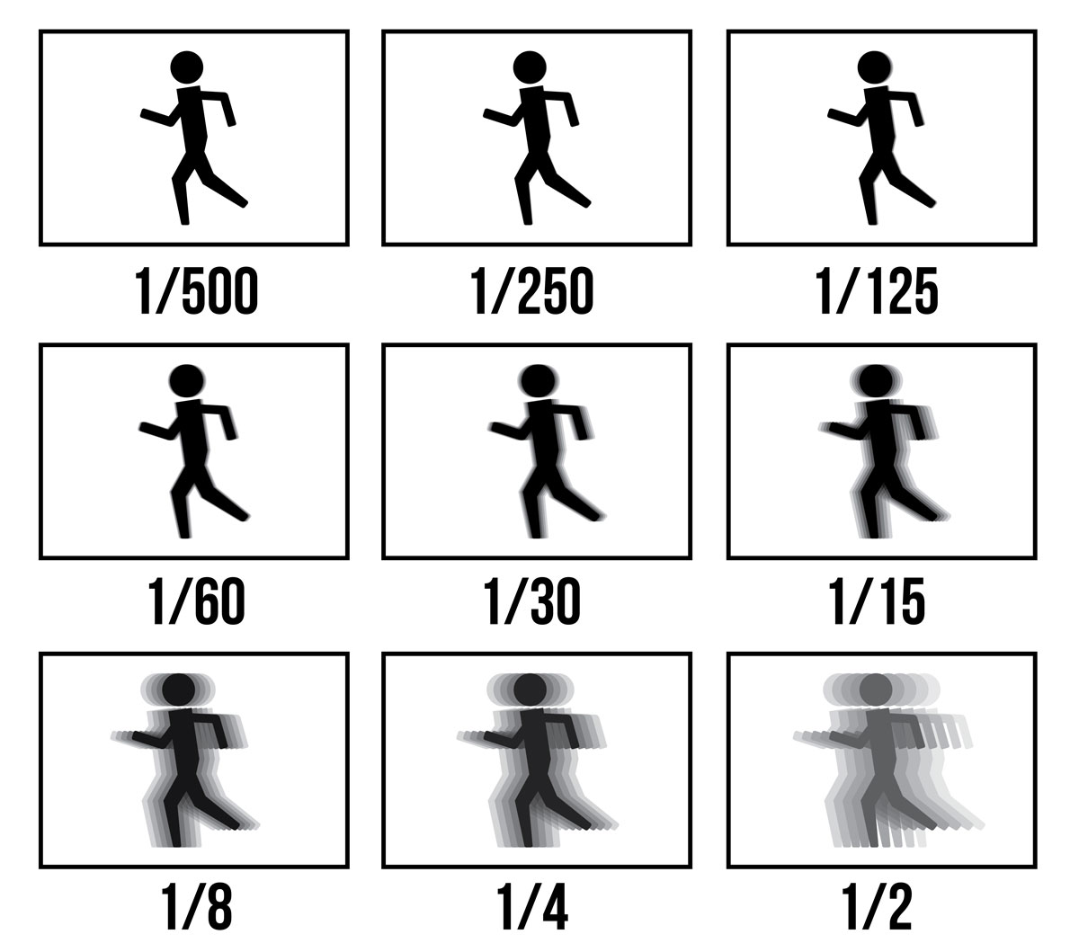Photo: creativelive.com

2.3 Final Words

Even though at first sight slow shutter may seem as a drawback at taking photos, but it can help to achieve spectacular presentation of a scene. Although it may help create enticing images, exposure is the other effect that need to be dealt because of the low speed of the shutter.

2.4 References

1. The Ultimate Guide To Learning Photography: Shutter Speed - creativelive.com
2. Introduction to Shutter Speed in Photography - Nasim Mansurov

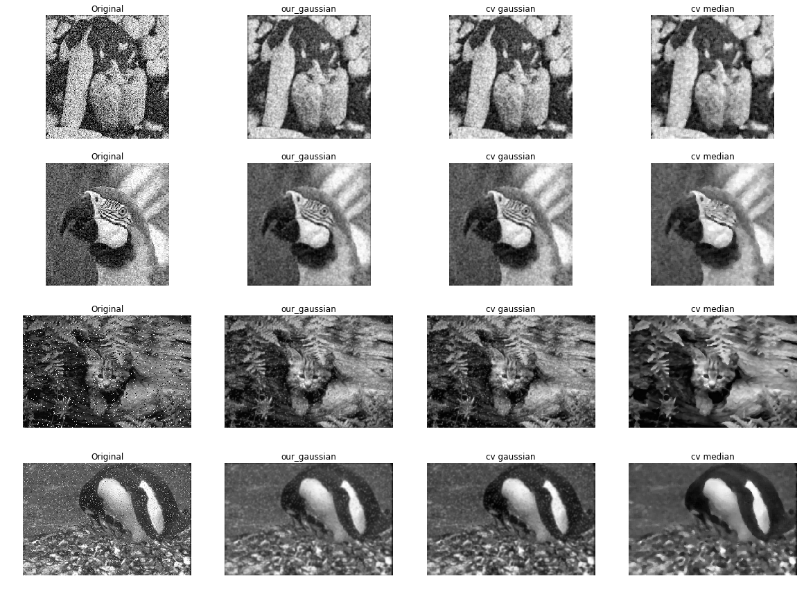
3 Histogram Equalization

In this section, the usage of histogram-equalization using open-cv and out implementation will be demonstrated. This section consists of following:

1. equalize_hist1 - open_cv
2. equalize_hist2 - Ours
   1. histogram
   2. equalize_hist2
3. T Plot

# necessary variables
import os
import cv2
import numpy as np
import matplotlib.pyplot as plt
%matplotlib inline

src_path = 'images/'
dst_path1 = 'results1/'
dst_path2 = 'results2/'
names = os.listdir(src_path)

L = 256

3.1 equalize_hist1(image)

def equalize_hist1(image):
    """
    Equalizes the histogram of the input grayscale image

    :param image: cv2 grayscale image
    :return: cv2 grayscale histogram equalized image
    """
    return cv2.equalizeHist(image)

fig, ax = plt.subplots(nrows=2, ncols=2, figsize=(15, 10))
fig2, ax2 = plt.subplots(nrows=2, ncols=2, figsize=(15, 10))
for idx, name in enumerate(names):
    # load image
    src_name = src_path + name
    image = cv2.imread(src_name, 0)

    # equalize histogram and write
    image1 = equalize_hist1(image)
    dst_name1 = dst_path1 + name
    cv2.imwrite(dst_name1, image1)

    # plotting
    ax[idx, 0].set_title('Original')
    ax[idx, 1].set_title('Equalized')
    ax2[idx, 0].set_title('Original')
    ax2[idx, 1].set_title('Equalized')
    ax[idx, 0].axis('off')
    ax[idx, 1].axis('off')

    ax[idx, 0].imshow(image, cmap='gray')
    ax[idx, 1].imshow(image1, cmap='gray')
    ax2[idx, 0].plot(cv2.calcHist([image], [0], None, [256], [0,256]))
    ax2[idx, 1].plot(cv2.calcHist([image1], [0], None, [256], [0,256]))

plt.show()

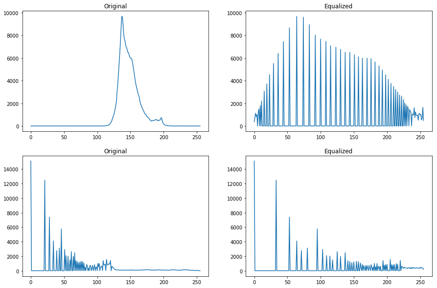
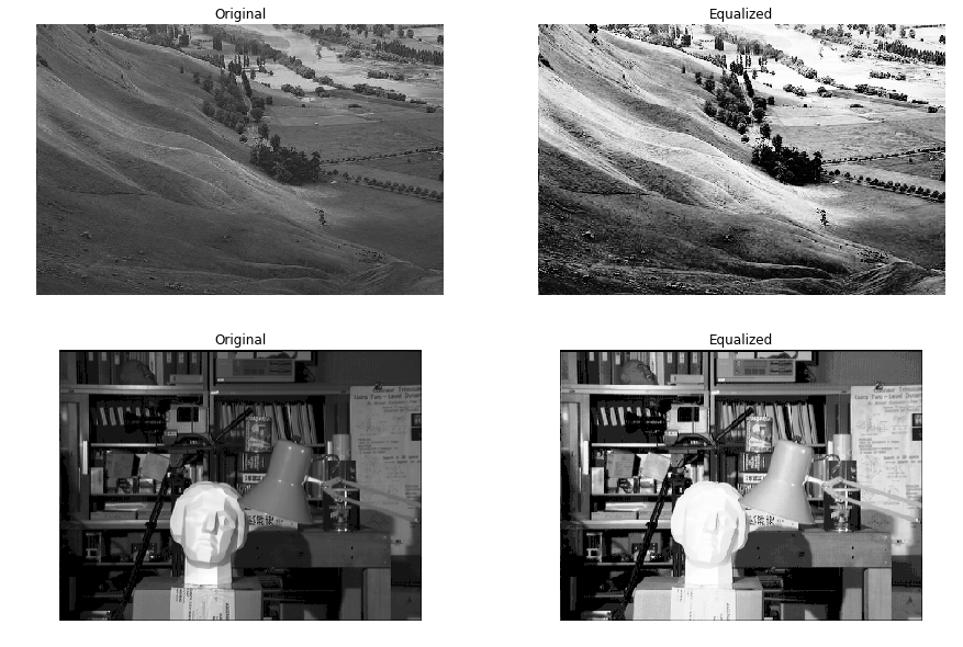
1. For the first example, as we can see, the image’s details has been improved intensely. The reason is the first image is a little dark and based on the histogram (upper left), almost all pixels have colors below 127, so by equalizing its histogram, we distribute the values between all the other possible colors, so as we can see in the equalized histogram (top right), the dark part of the image is now lighter.
2. In the second example, an immense amount of pixels are dark, so by equalizing its histogram, we introduce bigger values for pixels. The result for dark part of the image is completely acceptable because it is now light and details are easily detectable, but as we intensified the lighter ones too, we can see the head statue is completely light and details are gone.

3.2 equalize_hist2(image)

def histogram(image, L=256):
    """
    Gets and cv2 or numpy array image and acquire its histogram regarding provided number of levels

    :param image: A cv2 image or numpy ndarray
    :param L: Bins' count
    :return: A 1d np array
    """
    hist = np.zeros((L))
    for p in image.flatten():
        hist[p] += 1
    return hist

def cumulative_distribution_function(array):
    """
    calculates the cdf for given 1d np array (histogram)

    :param array: A 1d np array
    """
    cdf = np.zeros(array.shape)
    cdf[0] = array[0]
    for idx in range(1, len(array)):
        cdf[idx] += cdf[idx-1] + array[idx]
    return cdf

def equalize_hist2(image, L=256):
    """
    Equalizes the histogram of the input grayscale image

    :param image: cv2 grayscale image
    :return: cv2 grayscale histogram equalized image
    """
    # calculate histogram: Note that the value is different from numpy/open-cv one.
    hist = histogram(image, L)

    # calculate normalized cumulative distribution function
    cdf = cumulative_distribution_function(hist)
    cdf = cdf  / (image.shape[0]*image.shape[1]) * L-1
    cdf = cdf.astype('uint8')

    # equlize
    equalized = cdf[image]
    return equalized

fig, ax = plt.subplots(nrows=2, ncols=2, figsize=(15, 10))
fig2, ax2 = plt.subplots(nrows=2, ncols=2, figsize=(15, 10))
for idx, name in enumerate(names):
    # load image
    src_name = src_path + name
    image = cv2.imread(src_name, 0)

    # equalize histogram and write
    image2 = equalize_hist2(image)
    dst_name2 = dst_path2 + name
    cv2.imwrite(dst_name2, image2)

    # plotting
    ax[idx, 0].set_title('Original')
    ax[idx, 1].set_title('Equalized')
    ax[idx, 0].axis('off')
    ax[idx, 1].axis('off')
    ax2[idx, 0].set_title('Original')
    ax2[idx, 1].set_title('Equalized')
    ax3[0,idx].set_title('T of image "'+idx+'"')

    ax[idx, 0].imshow(image, cmap='gray')
    ax[idx, 1].imshow(image2, cmap='gray')

    ax2[idx, 0].plot(cv2.calcHist([image], [0], None, [256], [0,256]))
    ax2[idx, 1].plot(cv2.calcHist([image2], [0], None, [256], [0,256]))

plt.show()

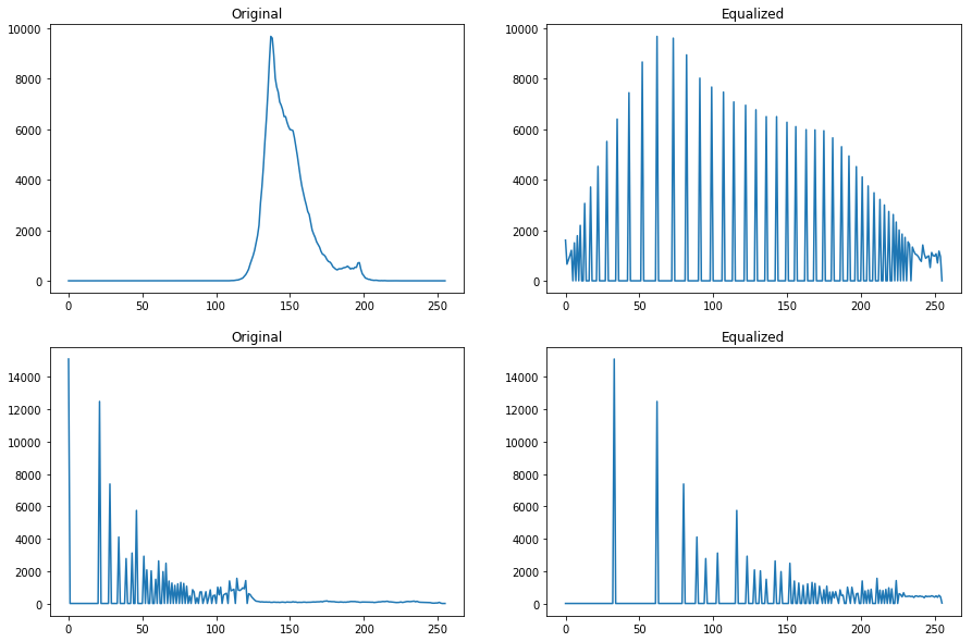
Note: The histogram of our implementation is different from the numpy/open-cv implementation and the reason is, their functions are general and works with different size of even varied widths and to achieve that, they use some kind of estimated distribution which can be found in official docs.

3.3 plotting T

In the end, we finalize the report by plotting the cdf values for both images.

src_name = src_path + names[0]
image = cv2.imread(src_name, 0)
cdf = cumulative_distribution_function(histogram(image))
cdf = (cdf  / (image.shape[0]*image.shape[1]) * L-1)
plt.title('T of first image')
plt.plot(cdf)

[<matplotlib.lines.Line2D at 0x1cce19b6668>]

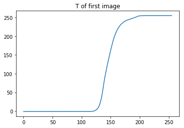
To explain the graph, based on first image’s histogram, we can say that almost all values are gathered around 150 so based on the plotted T, we can obtain that if the pixels are really dark range(0, 100), make them darker approximately, but if they are in the middle of concentration, intensify all of them. for instance, a pixel with value 120 can be converted to 10 but 150 can be 170 or something in the vicinity of that.

src_name = src_path + names[1]
image = cv2.imread(src_name, 0)
cdf = cumulative_distribution_function(histogram(image))
cdf = (cdf  / (image.shape[0]*image.shape[1]) * L-1)
plt.title('T of second image')
plt.plot(cdf)

[<matplotlib.lines.Line2D at 0x1cce3410e10>]

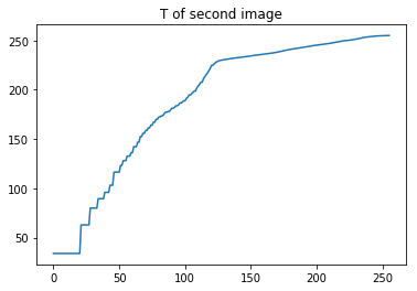
To explain this figure, we first need to mention the point that on the whole, our image is really dark except a small region at the middle, so our T function should focus on making the image lighter and as we can see this is happening. The result on the dark areas are promising but when image get lighter, this transform still intensifies the lightness. For instance, a pixel with value of 50 which is dark will be mapped to around 100 that is good but when the value is 200 it will be mapped to almost near to 255 which is unusual.