 Nikan
Nikan Convolutions, Separable Kernels and Gaussian Filter
This post consists of:
- Give short answers to below questions:
- How many zeros are needed to have a
sameconvolution over a256x256with a5x5filter? - What is the requirement of being Separable Kernels?
- How much speed-up will be up obtained if we use separated kernels of a
31x31kernel?
- How many zeros are needed to have a
- Write the separated kernels of the below filter and explain what they will do.
\begin{bmatrix}
-1 & 0 & 1
-2 & 0 & 2
-1 & 0 & 1 \end{bmatrix} - Instructions to obtain separated kernels
-
What is their jobs?
- Calculate below three tasks on paper:
- Compute the norm of following vectors:
\begin{equation}
x=
\begin{bmatrix}
1+j
2
1-j \end{bmatrix} , y= \begin{bmatrix} 1
-1
1 \end{bmatrix} \end{equation}
- Compute the norm of following vectors:
\begin{equation}
x=
\begin{bmatrix}
1+j
-
Calculate the inner product of
xandy. Are they orthonormal? -
Find degree between two following vectors: \begin{equation} x= \begin{bmatrix} 1
j
1-j \end{bmatrix} , y= \begin{bmatrix} -1
-j
j-1 \end{bmatrix} \end{equation} - Implement functions described in the following tasks:
- Implement
make_gaussianregarding 3.36 formula in reference book. Note thatsizeis same (size*size) and the output filter must be 2D with arbitrarysizeandstd. - Implement
convolve2dwith respect to the givenimageandkernel. You can use 3.35 formula in reference book. - Wrap up
medianandgaussianbuilt-in functions fromcv2in predefined functions. - Discuss the outputs using provided code and indicate the time they consumed.
- Implement
1 Short Answers
- How many zeros are needed to have a
sameconvolution over a256x256with a5x5filter? - What is the requirement of being Separable Kernels?
- How much speed-up will be up obtained if we use separated kernels of a
31x31kernel?
1.A
Firstly, We use following formula to calculate p or padding size:
\begin{equation}
x_n = \lfloor{x_o - f + 2p} \rfloor + 1
\end{equation}
Then we can get number of zeros using this formula: \begin{equation} nz = 4x_n + 4y_n + 4p^2 \end{equation}
import numpy as np
from scipy import ndimage
import matplotlib.pyplot as plt
image_size = 256
image_size_new = image_size
filter_size = 5
p = (image_size_new - image_size -1 + filter_size) // 2
x = np.ones((image_size, image_size))
f = np.ones((filter_size, filter_size))
x_padded = np.pad(x, p, mode='constant')
print(x_padded.shape)
print('Number of zeros from "np.pad" function:',len(x_padded.flatten()) - len(x_padded.nonzero()[0]))

nz = 4*image_size_new + 4*image_size_new + 4*p**2
print('Number of zeros:', nz)
(260, 260)
Number of zeros from "np.pad" function: 2064
Number of zeros: 2064
1.B Separable Kernels
We know the output matrices of the result of multiplying a row and a column matrix is rank 1. So the only requirement of being separable is that the kernel itself must be rank 1. Here is an example:
\begin{equation}
x=
\begin{bmatrix}
1
1
\end{bmatrix}
.
y=
\begin{bmatrix}
1 & 1 & 1
\end{bmatrix}=
\begin{bmatrix}
1 & 1 & 1
1 & 1 & 1
\end{bmatrix}
\end{equation}
print('Rank of aforementioned matrix:',np.linalg.matrix_rank([[1, 1, 1], [1, 1, 1]]))
Rank of aforementioned matrix: 1
1.C Speed Up of Separable Kernels
We follow this formula which exists in reference book: \begin{equation} speed = \frac{MNmn}{MNm+MNn} = \frac{mn}{m+n} \end{equation}
f = 31
speed = f*f / (f+f)
print('Speed up {}x'.format(speed))
Speed up 15.5x
2 Functionality of Separable Kernels of Kernel so-called Sobel
\begin{bmatrix}
-1 & 0 & 1
-2 & 0 & 2
-1 & 0 & 1
\end{bmatrix}
- Getting Separable Kernels
- Functionalities
2.A Getting Separable Kernels
- Choose any non-zero random number from the given matrix and call it
E - Get
E’s column as it is and call itV - Get
E’s row and call itr - Calculate
omega = r/E,Vandomegaare the kernels - You can get original kernel by calculating
w = V * omega.
kernel = np.array(
    [[-1, 0, 1],
     [-2, 0, 2],
     [-1, 0, 1]])
E_index = kernel.nonzero()[0][0], kernel.nonzero()[1][0]
V = kernel[:,E_index[1]].reshape(-1,1)
r = kernel[E_index[0],:].reshape(1,-1)
omega = r/kernel[E_index]
w = omega * V
print(w)
print(w.all() == kernel.all())
[[-1.  0.  1.]
 [-2.  0.  2.]
 [-1.  0.  1.]]
True
2.B Functionalities
- First Kernel
\begin{bmatrix}
-1
-2
-1 \end{bmatrix} - Second Kernel
\begin{bmatrix}
-1
0
1 \end{bmatrix}
2.B.a
\begin{bmatrix}
-1
-2
-1
\end{bmatrix}
r = 150
x = np.array([[r/5, r/5 , r],
            [r,r/5, r],
            [r, r/5 , r/5]
])
fig, ax = plt.subplots(nrows=2, ncols=1, figsize=(5, 8))
ax[0].imshow(x, cmap='gray')
x_conv = ndimage.convolve(x, [[1,2,1]])
x_conv[x_conv > 255] = 255
ax[1].imshow(x_conv, cmap='gray')
print(x)
print(x_conv)
[[  30.   30.  150.]
 [ 150.   30.  150.]
 [ 150.   30.   30.]]
[[ 120.  240.  255.]
 [ 255.  255.  255.]
 [ 255.  240.  120.]]
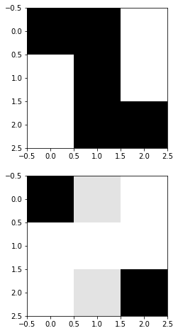
Smooths the image (decreases the frequency) for example decreasing the difference from 5x to 2x.
2.B.b
\begin{bmatrix}
-1
0
1
\end{bmatrix}
r = 20
x = np.array([[r, r , r/5],
            [r, r, r/5],
            [r, r , r/5]
])
fig, ax = plt.subplots(nrows=2, ncols=1, figsize=(5, 8))
ax[0].imshow(x, cmap='gray')
x_conv = ndimage.convolve(x, [[-1, 0, 1]])
x_conv[x_conv > 255] = 255
x_conv[x_conv < 0] = 0
ax[1].imshow(x_conv, cmap='gray')
print(x)
print(x_conv)
[[ 20.  20.   4.]
 [ 20.  20.   4.]
 [ 20.  20.   4.]]
[[  0.  16.  16.]
 [  0.  16.  16.]
 [  0.  16.  16.]]
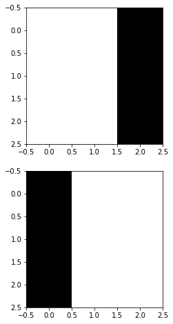
Intensifies the difference between low and high value pixels
3 Calculate on Paper:
-
Norm: \begin{equation} x= \begin{bmatrix} 1+j
2
1-j \end{bmatrix} , y= \begin{bmatrix} 1
-1
1 \end{bmatrix} \end{equation} -
Inner Product of
xandy. Orthonormal? -
Find Degree: \begin{equation} x= \begin{bmatrix} 1
j
1-j \end{bmatrix} , y= \begin{bmatrix} -1
-j
j-1 \end{bmatrix} \end{equation}
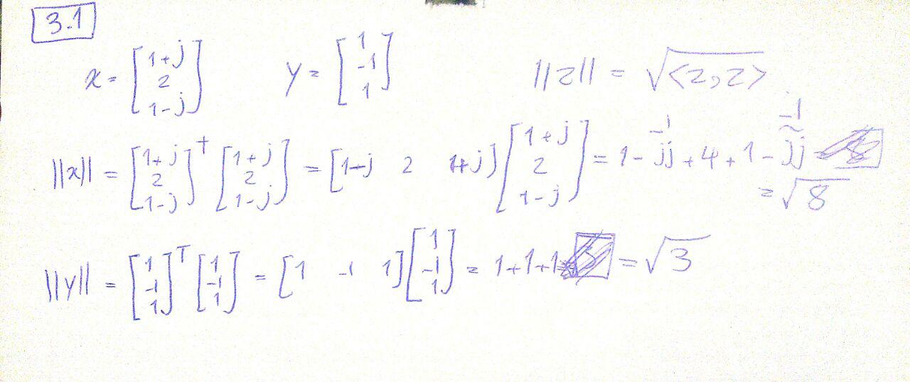
3.1 Norm
a = np.array([1+1j, 2, 1-1j]).reshape(-1, 1)
np.sqrt(np.vdot(a, a))
(2.8284271247461903+0j)
b = np.array([1, -1, 1]).reshape(-1, 1)
np.sqrt(np.vdot(b, b))
1.7320508075688772
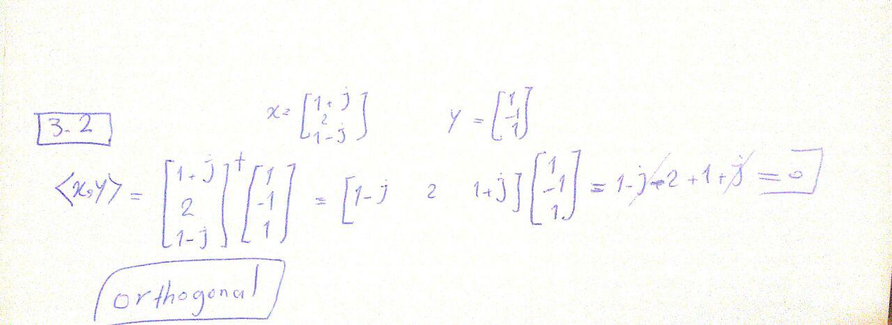
3.2 Inner Product
np.vdot(a, b)
0j
They are orthogonal not orthonormal.
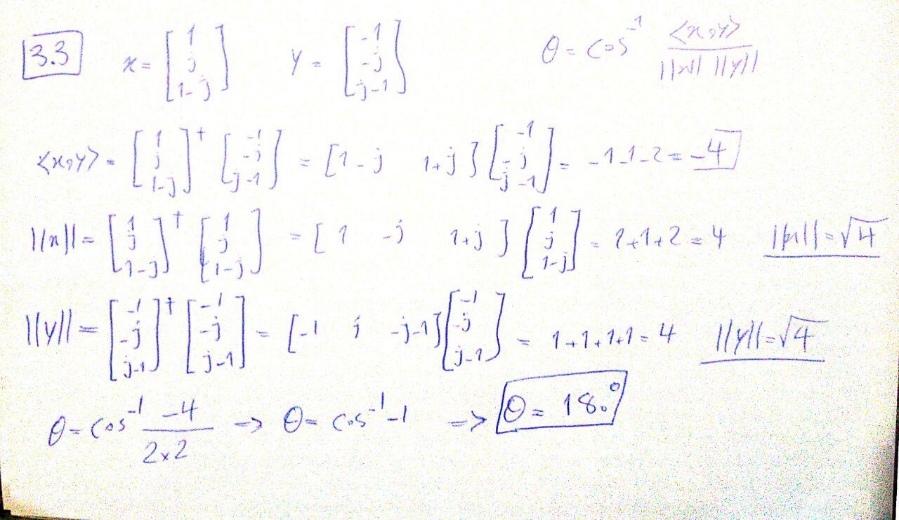
3.3 Find Degree
x = np.array([1, 1j, 1-1j]).reshape(-1, 1)
y = np.array([-1, -1j, 1j-1]).reshape(-1, 1)

xy = np.vdot(x, y)
x_norm = np.sqrt(np.vdot(x, x))
y_norm = np.sqrt(np.vdot(y, y))
theta = np.arccos(xy.real/(x_norm.real* y_norm.real))
theta = theta * 180 / np.pi
theta
180.0
4 Implementations
- Implement
make_gaussian(std, size) - Implement
convolve2d(image, kernel) - Implement
opencv_median_blur(image)fromcv2 - Implement
opencv_gaussian_blur(image, std, size)fromcv2 - Analyze
timeand Results
4.1 Implement make_gaussian(std, size)
def gaussian(r2, std=1):
    """
    Sample one instance from gaussian distribution regarding
    given squared-distance:r2, standard-deviation:std and general-constant:k

    :param r: squared distance from center of gaussian distribution
    :param std: standard deviation

    :return: A sampled number obtained from gaussian
    """
    return np.exp(-r2/(2.*std**2)) / (2.*np.pi*std**2)
def make_gaussian(size=5, std=1):
    """
    Creates a gaussian kernel regarding given size and std.
    Note that to define interval with respect to the size,
    I used linear space sampling which may has
    lower accuracy from renowned libraries.

    :param std: standard deviation value
    :param size: size of the output kernel
    :return: A gaussian kernel with size of (size*size)
    """
    size = int(size) // 2
    x, y = np.mgrid[-size:size+1, -size:size+1]
    distance = x**2+ y**2
    kernel = gaussian(r2=distance, std=std)
    return kernel

print(make_gaussian(5, 1))
[[ 0.00291502  0.01306423  0.02153928  0.01306423  0.00291502]
 [ 0.01306423  0.05854983  0.09653235  0.05854983  0.01306423]
 [ 0.02153928  0.09653235  0.15915494  0.09653235  0.02153928]
 [ 0.01306423  0.05854983  0.09653235  0.05854983  0.01306423]
 [ 0.00291502  0.01306423  0.02153928  0.01306423  0.00291502]]
4.2 Implement convolve2d(image, kernel)
def convolve2d(image, kernel):
    """
    Applies 2D convolution via provided kernel over given image

    :param image: input image in grayscale mode
    :param kernel: kernel of convolution
    :return: A convolved image with 'same' size using zero-padding
    """
    # you do not need to modify these, but feel free to implement however you know from scratch
    kernel       = np.flipud(np.fliplr(kernel))  # Flip the kernel, if it's symmetric it does not matter
    k = kernel.shape[0]
    padding      = (k - 1)
    offset       = padding // 2
    output       = np.zeros_like(image)
    # Add zero padding to the input image
    image_padded = np.zeros((image.shape[0] + padding, image.shape[1] + padding))
    image_padded[offset:-offset, offset:-offset] = image

    # implement the convolution inside the inner for loop
    for y in range(image.shape[0]):
        for x in range(image.shape[1]):
            output[y,x] = np.sum(kernel * image_padded[y:y+k, x:x+k])
    return output

x = np.random.randn(5, 5)
f = np.arange(9).reshape(3 ,3)
scipy_out = ndimage.convolve(x, f, mode='constant', cval=0)
our_out = convolve2d(x, f)

print('Results from scipy and out implementation are same? Answer:\n',scipy_out.astype('uint8') == our_out.astype('uint8'))
Results from scipy and out implementation are same? Answer:
 [[ True  True  True  True  True]
 [ True  True  True  True  True]
 [ True  True  True  True  True]
 [ True  True  True  True  True]
 [ True  True  True  True  True]]
4.3 Implement opencv_median_blur(image, size) from cv2
In Open CV, `size` argument also exists and it is mandatory which you omitted.
import cv2
def opencv_median_blur(image, size):
    """
    Applies median filter regarding given window `size`

    :param image: open cv or numpy ndarray image
    :param size: size of median kernel
    :return: An open cv image
    """
    return cv2.medianBlur(image, size)
4.4 Implement opencv_gaussian_blur(image, std, size) from cv2
def opencv_gaussian_blur(image, size, std):
    """
    Applies gaussian filter to smooth image

    :param image: Open cv or numpy ndarray image
    :param size: The size of gaussian filter
    :param std: if 0, it will be calculated automatically, otherwise for x and y should be indicated.
    :return: An open cv image
    """
    return cv2.GaussianBlur(src=image, ksize=(size, size), sigmaX=std, sigmaY=std)
4.5 Analyze time and Results
In Open CV, `size` argument also exists for `median` and it is mandatory which you omitted so I changed the `for` loop even though you said no to, to add `size=11` to `median`.
The reason I chose 11 is that in gaussian you used 11 too.
import os
import time
src_path = 'images_noisy/'
dst_path = 'images_filtered/'
names = os.listdir(src_path)

# Do not modify these for loops
for name in names:
    # load image
    src_name = src_path + name
    image = cv2.imread(src_name, cv2.IMREAD_GRAYSCALE)

    # gaussian blur using your implementation
    start = time.time()
    kernel1 = make_gaussian(std=1, size=11)
    blur1 = convolve2d(image, kernel1)
    dt1 = time.time() - start
    dst_name1 = dst_path + name + '.bmp'
    cv2.imwrite(dst_name1, blur1)

    # gaussian blur using opencv implementation
    start = time.time()
    blur2 = opencv_gaussian_blur(image, std=1, size=11)
    dt2 = time.time() - start
    dst_name2 = dst_path + name + '_CV.bmp'
    cv2.imwrite(dst_name2, blur2)

    # median blur
    start = time.time()
    blur3 = opencv_median_blur(image, 11)  ################# THIS CODE ONLY WORKS IF `SIZE` being provided.
    dt3 = time.time() - start
    dst_name3 = dst_path + name + '_median.bmp'
    cv2.imwrite(dst_name3, blur3)
    print('Our gaussian time:{}, opencv gaussian time:{}, opencv median time:{}'.format(dt1, dt2, dt3))
Our gaussian time:1.588090181350708, opencv gaussian time:0.0009992122650146484, opencv median time:0.004996776580810547
Our gaussian time:1.8719286918640137, opencv gaussian time:0.0, opencv median time:0.003996610641479492
Our gaussian time:2.5495409965515137, opencv gaussian time:0.0010004043579101562, opencv median time:0.009994029998779297
Our gaussian time:1.4371778964996338, opencv gaussian time:0.0009999275207519531, opencv median time:0.004997730255126953
Comparing Time Consumption
First of all, our implementation time is much bigger that open cv’s and it is completely obvious. If we want to compare gaussian, out convolution2d function has not been implemented efficiently which the main reason is the 2 for loops for iterating over image and computing convolution. The other reason is that opencv’s core is in C++ and we know that it is much faster (3x) even from efficient pure python code.
But if want to compare gaussian and median time, we can say that median operation is ordered and needs sorting every time and furthermore, it cannot be implemented using kernel logics which means most of the optimizations related to parallel computing or efficient vectorization will be lost, so that is why we can see an explosion about 10x increase in time.
Note: As you can see one of the times are 0.0 and that is because time module cannot handle very small numbers in small code snippets, so usually timeit module is preferred.
Comparing Quality
src_path = 'images_noisy/'
dst_path = 'images_filtered/'
names = os.listdir(src_path)

fig, ax = plt.subplots(nrows=4, ncols=4, figsize=(20, 15))
# Do not modify these for loops
for idx, name in enumerate(names):
    # load image
    src_name = src_path + name
    image = cv2.imread(src_name, cv2.IMREAD_GRAYSCALE)

    # gaussian blur using your implementation
    kernel1 = make_gaussian(std=1, size=11)
    blur1 = convolve2d(image, kernel1)

    # gaussian blur using opencv implementation
    blur2 = opencv_gaussian_blur(image, std=1, size=25)

    # median blur
    blur3 = opencv_median_blur(image, 5)

    # plotting
    ax[idx, 0].set_title('Original')
    ax[idx, 1].set_title('our_gaussian')
    ax[idx, 2].set_title('cv gaussian')
    ax[idx, 3].set_title('cv median')
    ax[idx, 0].axis('off')
    ax[idx, 1].axis('off')
    ax[idx, 2].axis('off')
    ax[idx, 3].axis('off')

    ax[idx, 0].imshow(image, cmap='gray')
    ax[idx, 1].imshow(blur1, cmap='gray')
    ax[idx, 2].imshow(blur2, cmap='gray')
    ax[idx, 3].imshow(blur3, cmap='gray')
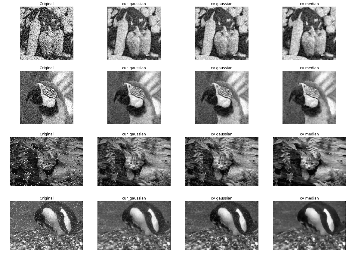
First two row of images correspond to the images with normal noise. So A gaussian blur can easily handle this kind of noises by reducing the frequency between pixels in the vicinity of each other without making image to blurry. But median, cannot find the good pixel to retain information without making the image completely blurry, because the noise is distributed almost between all values so median cannot do much and as you can see in the last column of the two first row, images are just blurry without removing noise.
But about the latter second rows, we can see the salt and pepper noise and this time, gaussian cannot do much because when it tries to decrease intensification, the output of convolution consists of 0 or 255 values and they will simply dominate other values so the output will be a blurry image without removing salt or peppers. They are still completely visible. But when we have such a noise in our images, we know they are minority in number so taking median, will focus on pixels that are more common in each window, so 0 or 255 values will not effect in median operation because they are almost rare in each window, so the output of images using this median filter will be blurry image without salt and peppers.
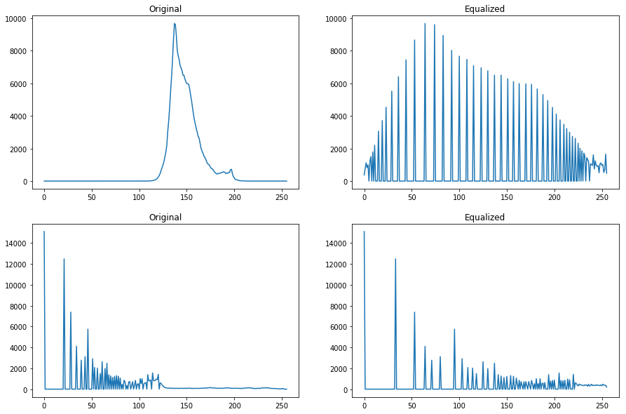 Shutter, Camera and Histogram Equalization