Morphological Operation, Hit-or-Miss, Textural Feature, Soft LBP, HOG, SVM and kNN

Morphological Operation, Hit-or-Miss, Textural Feature, Soft LBP, HOG, SVM and kNN

This post consists of:

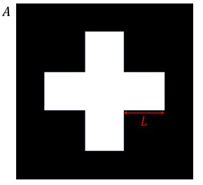
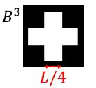
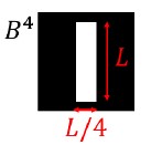
1. Consider this image and determine the type of morphological operation and structural element by defining its center:

A. B. C. D.

1. Given the sets as below images, draw the result of the given morphological operations:

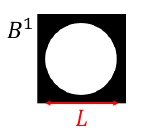
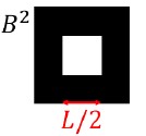
1. (A ⊝ B4) ⊕ B2
2. (A ⊝ B1) ⊕ B3
3. (A ⊕ B4) ⊕ B2
4. (A ⊕ B2) ⊝ B3

1. Do this tasks for this question:
   1. Hit-or-Miss operation has been explained in section 9.4 in the book (Gonsalez), explain it.
   2. Read this paper and compare LBP and Soft LBP.
2. Train and evaluate a model for Farsi handwritten digit recognition
   1. Use this dataset https://github.com/amir-saniyan/HodaDatasetReader
   2. Use Feature extraction such a texture
   3. Use SVM and kNN for learning process as mandatory classifiers
   4. Other classifiers (optional)
   5. Evaluate model using confusion matrix and average accuracy
   6. Compare results w.r.t. different features (optional)

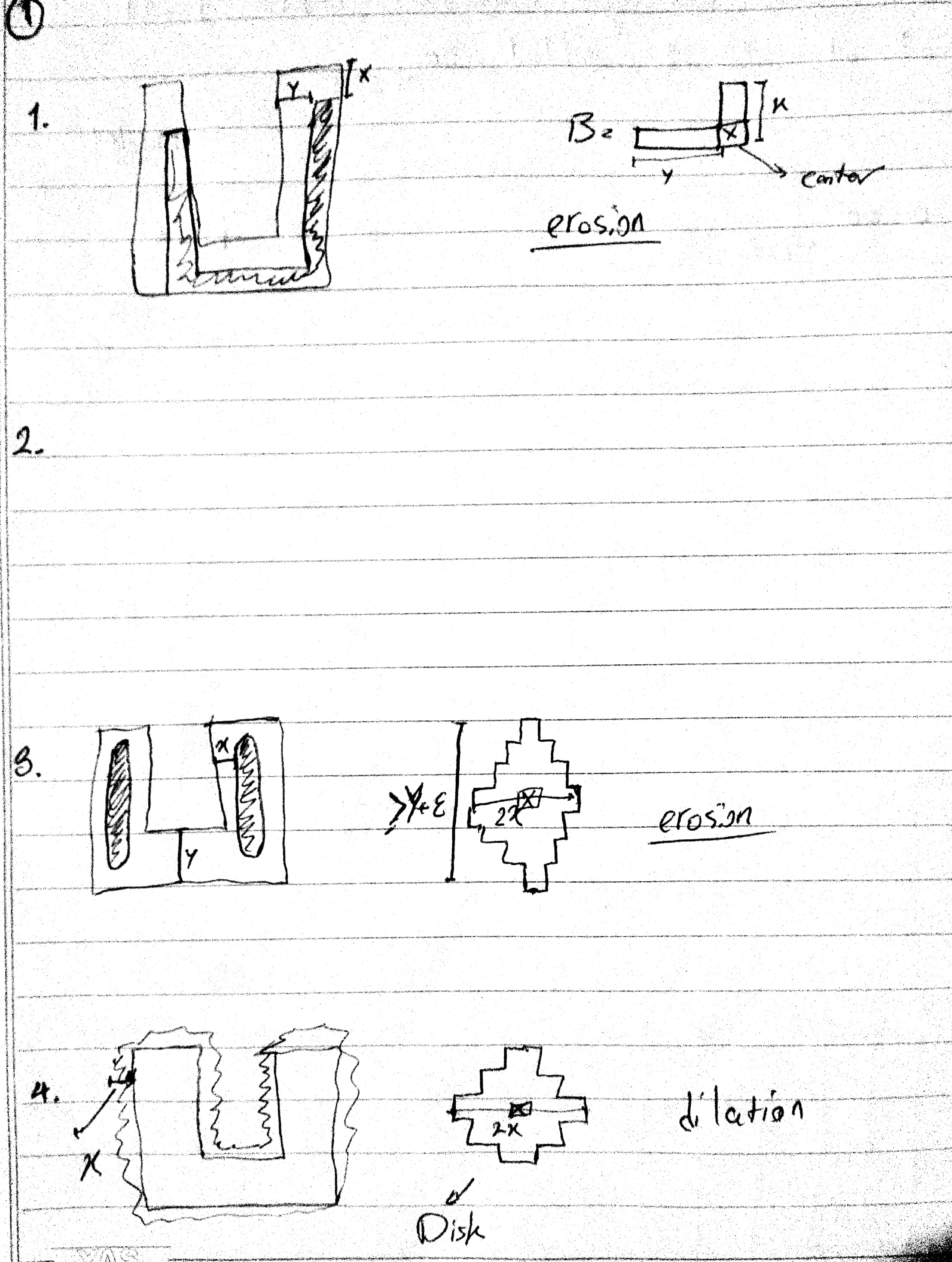
1 Consider this image and determine the type of morphological operation and structural element by defining its center:

1. 2. 3. 4.

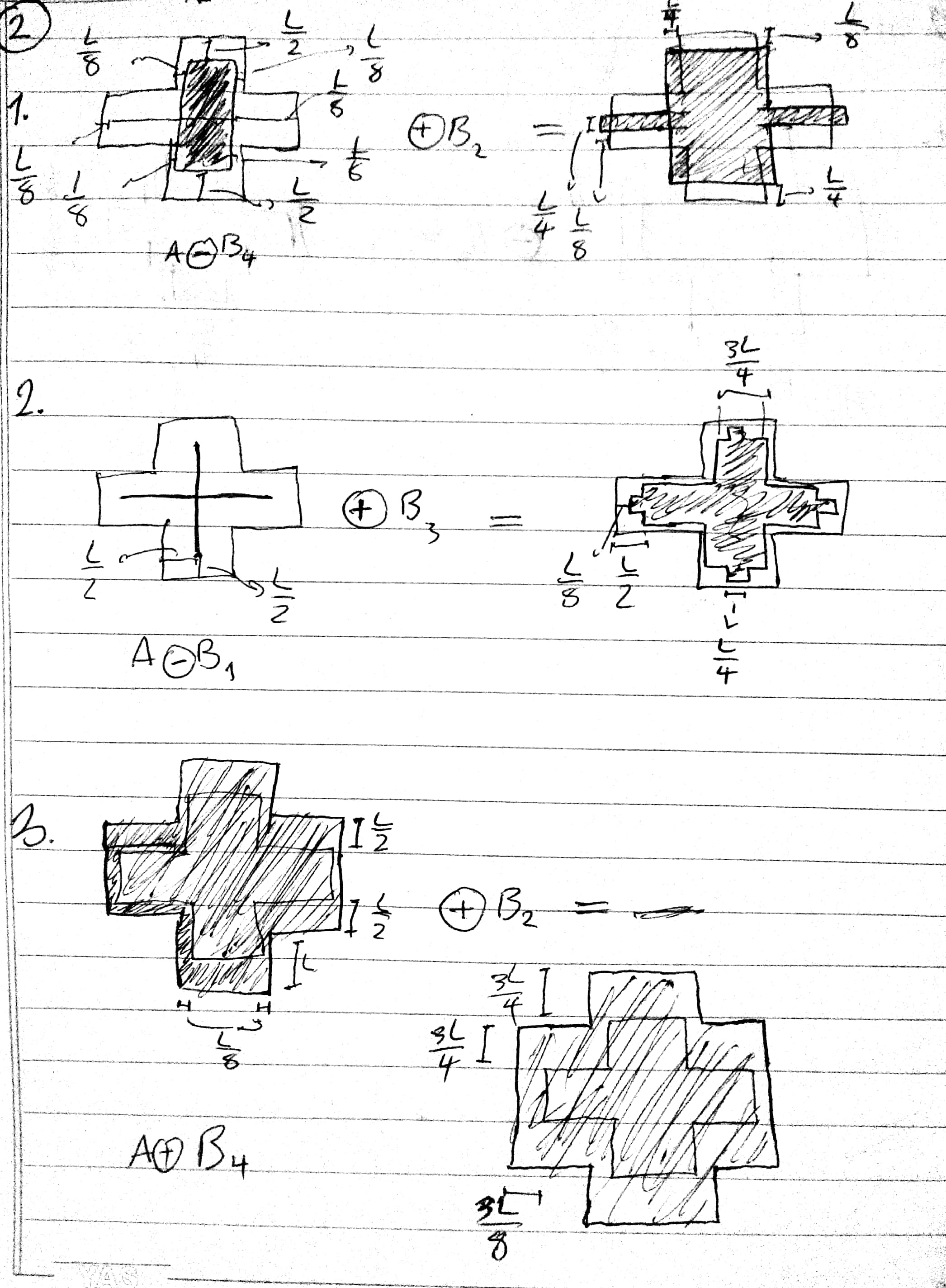
2 Given the sets as below images, draw the result of the given morphological operations:

1. (A ⊝ B4) ⊕ B2
2. (A ⊝ B1) ⊕ B3
3. (A ⊕ B4) ⊕ B2
4. (A ⊕ B2) ⊝ B3

3 Do this tasks for this question:

1. Hit-or-Miss operation has been explained in section 9.4 in the book (Gonzales), explain it.
2. Read this paper and compare LBP and Soft LBP.

3. A Hit-or-Miss Operator

First thing we need to know is that HOM is used for basic shape detection which works on binary images where 1s indicate foreground and 0s for background.

HOM uses two structural elements, one for foreground and one for background.

Here is the mathematical definition of it:

Intuitively, it says that foreground and background structural elements must match simultaneously. But we also can represent same operation using only one structural element, here is the mathematical definition:

In this situation, structural element B consists of both foreground and background pixels and that is why we need to do the operation simultaneously. In simple words, in erosion we just check for foreground elements but in this operation, we match foreground pixels of structural element with foreground pixels of image and at the same time wew also match background pixels of structural element with background pixels of image.

As a simple example, let’s say we want to find a dot in image. We need that it means that a single foreground pixel should be surrounded by many background pixels in all directions. So same structural element will be used and only would match when a single foreground pixel get surrounded by background pixels.

Here is 3 examples of this operation:

3.B Compare Soft LBP and LBP

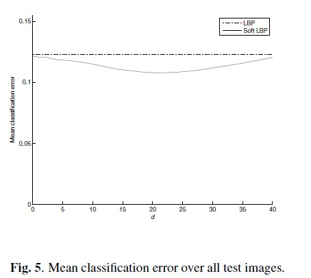
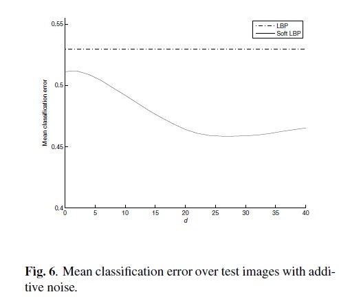
Soft LBP’s major characteristic is robustness against noises and continuous output w.r.t. inputs which also can work well on degraded images.

So let’s first talk about LBP itself and what makes it special. It is fast and invariant to gray-scale intensity changes which makes it tolerant against illumination changes which can be used for texture classification, face analysis, etc.

The possible problem of basic LBP could be the fixed thresholding regarding neighboring pixels where could make it very sensitive to noises.

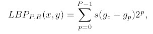
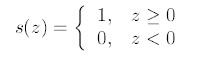
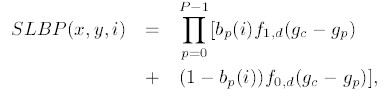
Basic LBP compare pixels in a 3x3 window and mark lower ones zero and vice versa. Finally, summing up by weighting to power of 2 would be our desired output. This operation and its thresholding window can be represented using below depictions where P is number of sampling points on a circle of radius of R:

Where the problem is the thresholding function which is as follow:

So as we knew it from the beginning the goal is to increase robustness via fuzzy membership function and here is the new defined functions where the parameter D controls the amount of fuzzification:

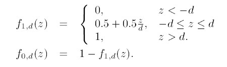
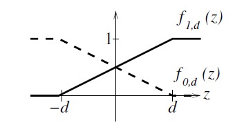
To build the histogram, now each pixel instead of contributing to only one bin where happens in basic LBP, now contributes to all bins regarding the membership function where sums up to 1 over all bins:

By using this membership functions, soft LBP looses one of the upsides of the basic LBP which is invariance to gray-level illumination. But the upside effect is that small changes introduces small effects too. On top of that, another issue affecting Soft LBP is that this method is computationally expensive because the contribution of the each pixel need to be computed w.r.t. all 2^P bins.

These result comparison could be great to finish explanation.

4 Train and evaluate a model for Farsi handwritten digit recognition

1. Use this dataset https://github.com/amir-saniyan/HodaDatasetReader
2. Use Features such a texture and geometry
3. Use SVM and kNN for learning process as mandatory classifiers
4. Evaluate model using confusion matrix and average accuracy
5. Compare results w.r.t. different features (optional)

!git clone https://github.com/amir-saniyan/HodaDatasetReader.git

Cloning into 'HodaDatasetReader'...
remote: Enumerating objects: 24, done.
remote: Total 24 (delta 0), reused 0 (delta 0), pack-reused 24
Unpacking objects: 100% (24/24), done.

import numpy as np
from matplotlib import pyplot as plt

from HodaDatasetReader.HodaDatasetReader import read_hoda_cdb, read_hoda_dataset

from sklearn.neighbors import KNeighborsClassifier
from sklearn.svm import LinearSVC, SVC
from sklearn.ensemble import AdaBoostClassifier, RandomForestClassifier
from sklearn.naive_bayes import GaussianNB
from sklearn.metrics import confusion_matrix

from skimage.feature import local_binary_pattern
import cv2

import pickle

4.A Use this dataset HodaDataset

train_images, train_labels = read_hoda_cdb('./HodaDatasetReader/DigitDB/Train 60000.cdb')
test_images, test_labels = read_hoda_cdb('./HodaDatasetReader/DigitDB/Test 20000.cdb')

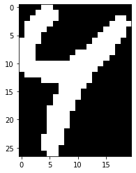
plt.imshow(train_images[0], cmap='gray')
print(train_labels[0])

6

4.B Feature Extraction

1. Geometry
2. Texture

4.B.a Geometry

def extract_geometrical_features(images):
    features = np.zeros((len(images), 5))

    for i in range(len(images)):

        try:
            im, contour, hierarchy = cv2.findContours(train_images[i], 1, 2)
            contour = contour[0]
            area = cv2.contourArea(contour)
            perimeter = cv2.arcLength(contour, True)
            convex_hull = cv2.convexHull(contour)
            convex_hull_area = cv2.contourArea(convex_hull)
            rect = cv2.minAreaRect(contour)
            _,_, w, h = cv2.boundingRect(contour)

            compactness = 4*np.pi*area/(perimeter**2)
            solidity = area / convex_hull_area
            eccentricity = rect[1][1] / rect[1][0]
            aspect_ratio = float(w)/float(h)
            extent = area / (w*h)
        except:
            pass

        features[i, 0] = compactness
        features[i, 1] = solidity
        features[i, 2] = eccentricity
        features[i, 3] = aspect_ratio
        features[i, 4] = extent

    return features

extract_geometrical_features(train_images[0:1])

array([[0.17906382, 0.46539792, 0.57727276, 0.74074074, 0.24907407]])

geometrical_features_train = extract_geometrical_features(train_images)
geometrical_features_test = extract_geometrical_features(test_images)

4.B.b Texture

Note as the size of images are not same, we need to find the maximum sized image and extend all other images to that size after extracting features. find_max_size can do this.

def find_max_size(images):
    return np.max([image.shape[0]*image.shape[1] for image in images])
max_len = np.max([find_max_size(train_images), find_max_size(test_images)])
max_len

2560

resized = cv2.resize(train_images[70], (32, 32), interpolation = cv2.INTER_AREA)
winSize = (16,16)
blockSize = (16,16)
blockStride = (8,8)
cellSize = (8,8)
nbins = 9
derivAperture = 1
winSigma = 4.
histogramNormType = 0
L2HysThreshold = 2.0000000000000001e-01
gammaCorrection = 0
nlevels = 64
hog = cv2.HOGDescriptor(winSize,blockSize,blockStride,cellSize,nbins,derivAperture,winSigma,
                        histogramNormType,L2HysThreshold,gammaCorrection,nlevels)
h = hog.compute(resized)
h = h.reshape(1, -1)

(324, 1)

def extract_textural_features(images, max_size, mode='lbp', feature_size=324):
    if mode=='lbp':
        # the reason of 16777215 magic number is that after calculating LBP, most of the values are this number so,
        # it's have been used to extend all LBP transform of images to same size
        features = np.ones((len(images), max_size)) * 16777215
        radius = 3
        n_points = 8 * radius
        for i in range(len(images)):
            features[i, :images[i].shape[0]*images[i].shape[1]] = local_binary_pattern(images[i], n_points, radius).flatten()
        return features
    elif mode=='hog':
        features = np.zeros((len(images), 324))  # for 32x32 image with this config result will be 324
        for idx, img in enumerate(images):
            img = cv2.resize(img, (32, 32), interpolation = cv2.INTER_AREA)
            winSize = (16,16)
            blockSize = (16,16)
            blockStride = (8,8)
            cellSize = (8,8)
            nbins = 9
            derivAperture = 1
            winSigma = 4.
            histogramNormType = 0
            L2HysThreshold = 2.0000000000000001e-01
            gammaCorrection = 0
            nlevels = 64
            hog = cv2.HOGDescriptor(winSize,blockSize,blockStride,cellSize,nbins,derivAperture,winSigma,
                                    histogramNormType,L2HysThreshold,gammaCorrection,nlevels)
            h = hog.compute(img)
            h = h.reshape(1, -1)
            features[idx,:] = h
        return features.astype(np.float16)
    else:
        pass

extract_textural_features(train_images[2:3], max_len)

array([[16777215., 16646145., 14614529., ..., 16777215., 16777215.,
        16777215.]])

extract_textural_features(train_images[2:3], None, 'hog').shape

(1, 324)

# LBP
textural_features_train = extract_textural_features(train_images, max_len)
textural_features_test = extract_textural_features(test_images, max_len)
textural_features_train = textural_features_train.astype(np.uint32)
textural_features_test = textural_features_test.astype(np.uint32)

# HOG
textural_features_hog_train = extract_textural_features(train_images, None, 'hog')
textural_features_hog_test = extract_textural_features(test_images, None, 'hog')

4.C Training

1. kNN
   1. Geometrical Features
   2. LBP Textural Features
   3. HOG Textural Features
2. Linear SVC
   1. Geometrical Features
   2. LBP Textural Features
   3. HOG Textural Features
3. Naive Bayes
   1. Geometrical Features
   2. LBP Textural Features
   3. HOG Textural Features
4. AdaBoost
   1. Geometrical Features
   2. LBP Textural Features
   3. HOG Textural Features
5. Random Forest
   1. Geometrical Features
   2. LBP Textural Features
   3. HOG Textural Features

4.C.a kNN Training

1. Geometric
2. LBP Textural
3. HOG Textural

4.C.a.i Geometric kNN

knn_geo = KNeighborsClassifier(n_neighbors=5, weights='distance')
knn_geo.fit(geometrical_features_train, train_labels)

KNeighborsClassifier(algorithm='auto', leaf_size=30, metric='minkowski',
                     metric_params=None, n_jobs=None, n_neighbors=5, p=2,
                     weights='distance')

4.C.a.ii LBP Textural kNN

knn_tex = KNeighborsClassifier(n_neighbors=5, weights='distance')
knn_tex.fit(textural_features_train, train_labels)

KNeighborsClassifier(algorithm='auto', leaf_size=30, metric='minkowski',
                     metric_params=None, n_jobs=None, n_neighbors=5, p=2,
                     weights='distance')

4.C.a.iii HOG Textural kNN

knn_tex_hog = KNeighborsClassifier(n_neighbors=5, weights='distance')
knn_tex_hog.fit(textural_features_hog_train, train_labels)

KNeighborsClassifier(algorithm='auto', leaf_size=30, metric='minkowski',
                     metric_params=None, n_jobs=None, n_neighbors=5, p=2,
                     weights='distance')

pickle.dump(knn_geo, open('knn_geo.model', 'wb'))
pickle.dump(knn_tex, open('knn_tex.model', 'wb'))

4.C.b Linear SVC Training

1. Geometric
2. LBP Textural
3. HOG Textural

4.C.b.i Geometrical Linear SVC

linear_svc_geo = LinearSVC(max_iter=20000)
linear_svc_geo.fit(geometrical_features_train, train_labels)

LinearSVC(C=1.0, class_weight=None, dual=True, fit_intercept=True,
          intercept_scaling=1, loss='squared_hinge', max_iter=20000,
          multi_class='ovr', penalty='l2', random_state=None, tol=0.0001,
          verbose=0)

4.C.b.ii LBP Textural Linear SVC

linear_svc_tex = LinearSVC(max_iter=500, tol=1e-4)
linear_svc_tex.fit(textural_features_train, train_labels)

/usr/local/lib/python3.6/dist-packages/sklearn/svm/base.py:929: ConvergenceWarning: Liblinear failed to converge, increase the number of iterations.
  "the number of iterations.", ConvergenceWarning)





LinearSVC(C=1.0, class_weight=None, dual=True, fit_intercept=True,
          intercept_scaling=1, loss='squared_hinge', max_iter=500,
          multi_class='ovr', penalty='l2', random_state=None, tol=0.0001,
          verbose=0)

4.C.b.iii HOG Textural Linear SVC

linear_svc_tex_hog = LinearSVC(max_iter=500)
linear_svc_tex_hog.fit(textural_features_hog_train, train_labels)

LinearSVC(C=1.0, class_weight=None, dual=True, fit_intercept=True,
          intercept_scaling=1, loss='squared_hinge', max_iter=500,
          multi_class='ovr', penalty='l2', random_state=None, tol=0.0001,
          verbose=0)

4.C.d Naive Bayes Training

1. Geometric
2. LBP Textural
3. HOG Textural

4.C.d.i Geometrical Naive Bayes

gnb_geo = GaussianNB()
gnb_geo.fit(geometrical_features_train, train_labels)

GaussianNB(priors=None, var_smoothing=1e-09)

4.C.d.ii LBP Textural Naive Bayes

gnb_tex = GaussianNB()
gnb_tex.fit(textural_features_train, train_labels)

GaussianNB(priors=None, var_smoothing=1e-09)

4.C.d.iii HOG Textural Naive Bayes

gnb_tex_hog = GaussianNB()
gnb_tex_hog.fit(textural_features_hog_train, train_labels)

GaussianNB(priors=None, var_smoothing=1e-09)

4.C.e AdaBoost Training

1. Geometric
2. LBP Textural
3. HOG Textural

4.C.e.i Geometrical AdaBoost

adaboost_geo = AdaBoostClassifier(n_estimators=100)  # using decision tree depth=1
adaboost_geo.fit(geometrical_features_train, train_labels)

AdaBoostClassifier(algorithm='SAMME.R', base_estimator=None, learning_rate=1.0,
                   n_estimators=100, random_state=None)

4.C.e.ii LBP Textural AdaBoost

adaboost_tex = AdaBoostClassifier(n_estimators=100)  # using decision tree depth=1
adaboost_tex.fit(textural_features_train, train_labels)

AdaBoostClassifier(algorithm='SAMME.R', base_estimator=None, learning_rate=1.0,
                   n_estimators=100, random_state=None)

4.C.e.iii HOG Textural AdaBoost

adaboost_tex_hog = AdaBoostClassifier(n_estimators=100)  # using decision tree depth=1
adaboost_tex_hog.fit(textural_features_hog_train, train_labels)

AdaBoostClassifier(algorithm='SAMME.R', base_estimator=None, learning_rate=1.0,
                   n_estimators=100, random_state=None)

4.C.f RandomForest Training

1. Geometric
2. HOG Textural

4.C.f.i Geometrical Random Forest

randomforest_geo = RandomForestClassifier(min_samples_leaf=5, n_estimators=100)
randomforest_geo.fit(geometrical_features_train, train_labels)

RandomForestClassifier(bootstrap=True, class_weight=None, criterion='gini',
                       max_depth=None, max_features='auto', max_leaf_nodes=None,
                       min_impurity_decrease=0.0, min_impurity_split=None,
                       min_samples_leaf=5, min_samples_split=2,
                       min_weight_fraction_leaf=0.0, n_estimators=100,
                       n_jobs=None, oob_score=False, random_state=None,
                       verbose=0, warm_start=False)

4.C.f.ii HOG Textural Random Forest

randomforest_tex_hog = RandomForestClassifier(n_estimators=100)  # using decision tree depth=1
randomforest_tex_hog.fit(textural_features_hog_train, train_labels)

RandomForestClassifier(bootstrap=True, class_weight=None, criterion='gini',
                       max_depth=None, max_features='auto', max_leaf_nodes=None,
                       min_impurity_decrease=0.0, min_impurity_split=None,
                       min_samples_leaf=1, min_samples_split=2,
                       min_weight_fraction_leaf=0.0, n_estimators=100,
                       n_jobs=None, oob_score=False, random_state=None,
                       verbose=0, warm_start=False)

4.D Evaluation

1. kNN
2. Linear SVC
3. RBF SVC
4. Naive Bayes
5. AdaBoost
6. Random Forest

def draw_confusion_matrix(y_true, y_pred, classes=None, normalize=True, title=None, cmap=plt.cm.Blues):
    acc = np.sum(y_true == y_pred) / len(y_true)
    print('Accuracy = {}'.format(acc))

    cm = confusion_matrix(y_true, y_pred)
    if normalize:
        cm = cm.astype('float') / cm.sum(axis=1)[:, np.newaxis]
    print('Confusion Matrix = \n{}'.format(np.round(cm, 3)))

    if classes is None:
        classes = [str(i) for i in range(len(np.unique(y_true)))]

    if not title:
        if normalize:
            title = 'Normalized confusion matrix'
        else:
            title = 'Confusion matrix, without normalization'

    fig, ax = plt.subplots()
    im = ax.imshow(cm, interpolation='nearest', cmap=cmap)
    ax.figure.colorbar(im, ax=ax)
    # We want to show all ticks...
    ax.set(xticks=np.arange(cm.shape[1]),
           yticks=np.arange(cm.shape[0]),
           # ... and label them with the respective list entries
           xticklabels=classes, yticklabels=classes,
           title=title,
           ylabel='True label',
           xlabel='Predicted label')

    # Rotate the tick labels and set their alignment.
    plt.setp(ax.get_xticklabels(), rotation=45, ha="right",
             rotation_mode="anchor")

    # Loop over data dimensions and create text annotations.
    fmt = '.2f' if normalize else 'd'
    thresh = cm.max() / 2.
    for i in range(cm.shape[0]):
        for j in range(cm.shape[1]):
            ax.text(j, i, format(cm[i, j], fmt),
                    ha="center", va="center",
                    color="white" if cm[i, j] > thresh else "black")
    fig.tight_layout()
    plt.show()
    return ax

4.D.a kNN Evaluation

1. Geometrical
2. LBP Textural
3. HOG Textural

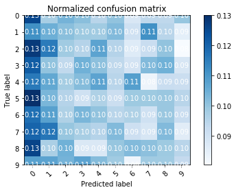
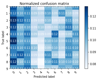
4.D.a.i Geometric kNN

pred = knn_geo.predict(geometrical_features_test)
draw_confusion_matrix(test_labels, pred)

Accuracy = 0.10095
Confusion Matrix =
[[0.126 0.098 0.104 0.102 0.095 0.1   0.088 0.094 0.094 0.1  ]
 [0.112 0.105 0.102 0.099 0.098 0.102 0.09  0.112 0.095 0.085]
 [0.128 0.116 0.098 0.096 0.108 0.096 0.086 0.092 0.1   0.08 ]
 [0.122 0.1   0.094 0.104 0.101 0.094 0.09  0.102 0.104 0.088]
 [0.116 0.106 0.098 0.102 0.108 0.095 0.108 0.083 0.092 0.092]
 [0.13  0.104 0.096 0.09  0.096 0.092 0.099 0.099 0.1   0.095]
 [0.118 0.108 0.096 0.104 0.1   0.095 0.096 0.09  0.1   0.092]
 [0.12  0.116 0.1   0.098 0.096 0.102 0.091 0.088 0.102 0.086]
 [0.126 0.097 0.104 0.088 0.088 0.1   0.102 0.101 0.099 0.095]
 [0.108 0.108 0.104 0.108 0.102 0.098 0.082 0.098 0.098 0.093]]

<matplotlib.axes._subplots.AxesSubplot at 0x7ff5cb693da0>

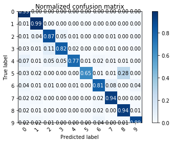
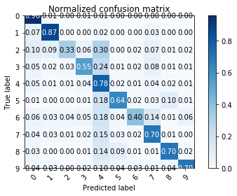
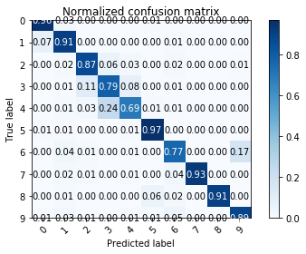
4.D.a.ii LBP Textural kNN

# takes about 100 mins!!!
pred = knn_tex.predict(textural_features_test)
draw_confusion_matrix(test_labels, pred)

Accuracy = 0.8665
Confusion Matrix =
[[0.988 0.004 0.    0.    0.    0.004 0.    0.002 0.    0.001]
 [0.006 0.988 0.002 0.    0.    0.    0.002 0.    0.    0.002]
 [0.015 0.036 0.874 0.051 0.01  0.    0.004 0.007 0.    0.002]
 [0.025 0.014 0.106 0.821 0.023 0.    0.002 0.006 0.002 0.   ]
 [0.07  0.01  0.05  0.052 0.77  0.006 0.024 0.008 0.006 0.001]
 [0.028 0.022 0.002 0.001 0.002 0.652 0.011 0.006 0.276 0.002]
 [0.038 0.008 0.014 0.002 0.008 0.003 0.806 0.076 0.004 0.041]
 [0.02  0.016 0.002 0.    0.    0.    0.022 0.935 0.    0.004]
 [0.02  0.007 0.001 0.    0.    0.    0.022 0.002 0.939 0.01 ]
 [0.022 0.02  0.007 0.    0.    0.002 0.043 0.003 0.009 0.892]]

<matplotlib.axes._subplots.AxesSubplot at 0x7fd45d24b320>

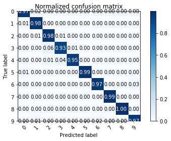
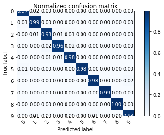
4.D.a.iii HOG Textural kNN

pred = knn_tex_hog.predict(textural_features_hog_test)
draw_confusion_matrix(test_labels, pred)

Accuracy = 0.97215
Confusion Matrix =
[[0.971 0.023 0.    0.    0.    0.004 0.    0.001 0.    0.   ]
 [0.014 0.982 0.002 0.    0.    0.    0.    0.    0.    0.   ]
 [0.    0.006 0.977 0.014 0.002 0.    0.    0.    0.    0.001]
 [0.    0.    0.056 0.928 0.013 0.002 0.    0.    0.    0.   ]
 [0.    0.    0.014 0.037 0.949 0.    0.    0.    0.    0.   ]
 [0.008 0.002 0.002 0.    0.    0.986 0.    0.    0.002 0.   ]
 [0.    0.    0.    0.    0.001 0.002 0.966 0.    0.    0.03 ]
 [0.    0.002 0.    0.    0.    0.    0.002 0.994 0.    0.   ]
 [0.    0.002 0.    0.    0.    0.    0.    0.    0.998 0.   ]
 [0.001 0.009 0.001 0.    0.    0.001 0.017 0.    0.001 0.97 ]]

<matplotlib.axes._subplots.AxesSubplot at 0x7fef8f16a588>

4.D.b Linear SVC Evaluation

1. Geometrical
2. LBP Textural
3. HOG Textural

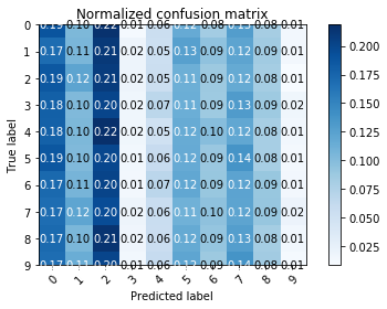
4.D.b.i Geometrical Linear SVC

pred = linear_svc_geo.predict(geometrical_features_test)
draw_confusion_matrix(test_labels, pred)

Accuracy = 0.09935
Confusion Matrix =
[[0.189 0.104 0.216 0.011 0.055 0.116 0.084 0.128 0.082 0.014]
 [0.17  0.106 0.21  0.018 0.054 0.126 0.094 0.122 0.086 0.014]
 [0.186 0.122 0.208 0.018 0.054 0.112 0.088 0.118 0.083 0.008]
 [0.18  0.102 0.2   0.016 0.068 0.113 0.087 0.13  0.086 0.016]
 [0.179 0.104 0.218 0.016 0.051 0.116 0.099 0.12  0.082 0.015]
 [0.187 0.102 0.2   0.015 0.06  0.116 0.09  0.136 0.081 0.013]
 [0.172 0.107 0.202 0.014 0.068 0.12  0.09  0.123 0.09  0.014]
 [0.169 0.121 0.195 0.018 0.057 0.111 0.095 0.122 0.091 0.02 ]
 [0.172 0.104 0.215 0.018 0.056 0.118 0.092 0.128 0.083 0.015]
 [0.168 0.114 0.201 0.014 0.06  0.121 0.088 0.138 0.084 0.011]]

<matplotlib.axes._subplots.AxesSubplot at 0x7ff5cb01e3c8>

4.D.b.ii LBP Textural Linear SVC

# note that because of colab's 12 hours time limitation SVC failed to converge so this result is not optimal.
pred = linear_svc_tex.predict(textural_features_test)
draw_confusion_matrix(test_labels, pred)

Accuracy = 0.66145
Confusion Matrix =
[[0.957 0.014 0.    0.008 0.012 0.001 0.002 0.001 0.002 0.003]
 [0.07  0.868 0.004 0.001 0.016 0.001 0.003 0.034 0.002 0.002]
 [0.104 0.088 0.327 0.06  0.304 0.003 0.018 0.072 0.006 0.019]
 [0.05  0.02  0.026 0.548 0.237 0.012 0.016 0.076 0.006 0.008]
 [0.054 0.01  0.012 0.038 0.784 0.016 0.015 0.042 0.02  0.008]
 [0.006 0.001 0.001 0.006 0.178 0.639 0.023 0.03  0.1   0.014]
 [0.056 0.034 0.035 0.05  0.176 0.036 0.399 0.136 0.014 0.063]
 [0.036 0.026 0.015 0.022 0.151 0.028 0.019 0.696 0.006 0.003]
 [0.03  0.002 0.    0.007 0.141 0.09  0.006 0.007 0.7   0.016]
 [0.043 0.026 0.002 0.016 0.095 0.036 0.033 0.013 0.039 0.696]]

<matplotlib.axes._subplots.AxesSubplot at 0x7fd45a5f4fd0>

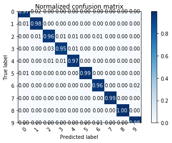
4.D.b.iii HOG Textural Linear SVC

pred = linear_svc_tex_hog.predict(textural_features_hog_test)
draw_confusion_matrix(test_labels, pred)

Accuracy = 0.9765
Confusion Matrix =
[[0.971 0.022 0.    0.    0.002 0.004 0.001 0.001 0.    0.   ]
 [0.012 0.982 0.    0.    0.002 0.002 0.002 0.    0.    0.   ]
 [0.    0.011 0.964 0.008 0.008 0.    0.006 0.002 0.    0.002]
 [0.    0.    0.028 0.953 0.015 0.002 0.    0.    0.    0.002]
 [0.    0.001 0.008 0.013 0.973 0.002 0.001 0.    0.    0.002]
 [0.006 0.002 0.    0.    0.002 0.988 0.    0.    0.    0.   ]
 [0.    0.003 0.002 0.002 0.003 0.002 0.962 0.001 0.002 0.022]
 [0.    0.002 0.002 0.    0.    0.    0.003 0.992 0.    0.   ]
 [0.    0.001 0.    0.    0.    0.    0.    0.    0.997 0.   ]
 [0.    0.004 0.001 0.002 0.002 0.001 0.008 0.    0.    0.982]]

<matplotlib.axes._subplots.AxesSubplot at 0x7fef8f000e48>

4.E.d Naive Bayes Evaluation

1. Geometric
2. LBP Textural
3. HOG Textural

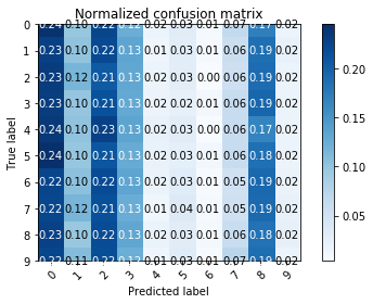
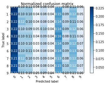
4.E.d.i Geometrical Naive Bayes

pred = gnb_geo.predict(geometrical_features_test)
draw_confusion_matrix(test_labels, pred)

Accuracy = 0.0984
Confusion Matrix =
[[0.242 0.098 0.223 0.124 0.017 0.031 0.008 0.066 0.17  0.019]
 [0.229 0.101 0.221 0.133 0.015 0.03  0.006 0.058 0.186 0.022]
 [0.233 0.116 0.206 0.131 0.018 0.029 0.004 0.056 0.188 0.019]
 [0.232 0.099 0.213 0.13  0.018 0.024 0.012 0.061 0.194 0.019]
 [0.236 0.102 0.228 0.134 0.021 0.031 0.004 0.062 0.166 0.017]
 [0.244 0.098 0.21  0.126 0.02  0.026 0.01  0.062 0.185 0.018]
 [0.224 0.104 0.218 0.134 0.02  0.032 0.006 0.052 0.192 0.02 ]
 [0.222 0.116 0.215 0.126 0.013 0.036 0.007 0.054 0.19  0.022]
 [0.228 0.098 0.218 0.132 0.02  0.031 0.008 0.06  0.182 0.023]
 [0.223 0.109 0.217 0.124 0.014 0.032 0.006 0.072 0.186 0.016]]

<matplotlib.axes._subplots.AxesSubplot at 0x7fd45a454940>

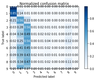
4.E.d.ii LBP Textural Naive Bayes

pred = gnb_tex.predict(textural_features_test)
draw_confusion_matrix(test_labels, pred)

Accuracy = 0.1524
Confusion Matrix =
[[0.988 0.01  0.002 0.    0.    0.    0.    0.    0.    0.   ]
 [0.849 0.136 0.014 0.    0.    0.    0.    0.    0.    0.   ]
 [0.206 0.556 0.219 0.    0.002 0.004 0.002 0.    0.011 0.   ]
 [0.032 0.282 0.556 0.012 0.018 0.015 0.012 0.001 0.071 0.   ]
 [0.038 0.342 0.492 0.01  0.016 0.021 0.008 0.    0.074 0.   ]
 [0.016 0.254 0.562 0.002 0.008 0.037 0.002 0.    0.12  0.   ]
 [0.055 0.41  0.451 0.004 0.01  0.016 0.002 0.    0.048 0.004]
 [0.09  0.387 0.43  0.016 0.01  0.026 0.006 0.002 0.034 0.   ]
 [0.053 0.342 0.466 0.    0.012 0.018 0.    0.    0.109 0.   ]
 [0.051 0.467 0.371 0.    0.014 0.014 0.002 0.    0.079 0.002]]

<matplotlib.axes._subplots.AxesSubplot at 0x7fd45a2d06d8>

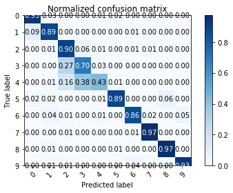
4.E.d.iii HOG Textural Naive Bayes

pred = gnb_tex_hog.predict(textural_features_hog_test)
draw_confusion_matrix(test_labels, pred)

Accuracy = 0.8686
Confusion Matrix =
[[0.956 0.027 0.    0.    0.003 0.009 0.004 0.    0.    0.   ]
 [0.07  0.911 0.004 0.    0.002 0.001 0.011 0.    0.    0.002]
 [0.    0.018 0.868 0.062 0.026 0.    0.018 0.002 0.    0.006]
 [0.    0.005 0.113 0.794 0.077 0.    0.008 0.    0.    0.004]
 [0.003 0.012 0.028 0.242 0.694 0.01  0.008 0.    0.    0.002]
 [0.01  0.01  0.    0.    0.01  0.968 0.002 0.    0.    0.   ]
 [0.001 0.036 0.014 0.    0.008 0.004 0.766 0.    0.    0.172]
 [0.001 0.016 0.008 0.    0.006 0.    0.036 0.932 0.    0.   ]
 [0.    0.012 0.    0.    0.002 0.058 0.022 0.    0.906 0.   ]
 [0.006 0.028 0.006 0.    0.01  0.012 0.047 0.    0.002 0.89 ]]

<matplotlib.axes._subplots.AxesSubplot at 0x7fef8c69fc50>

4.C.e AdaBoost Evaluation

1. Geometric
2. LBP Textural
3. HOG Textural

4.E.e.i Geometrical AdaBoost

pred = adaboost_geo.predict(geometrical_features_test)
draw_confusion_matrix(test_labels, pred)

Accuracy = 0.101
Confusion Matrix =
[[0.228 0.1   0.108 0.041 0.078 0.044 0.149 0.08  0.114 0.058]
 [0.22  0.104 0.104 0.042 0.078 0.04  0.146 0.088 0.124 0.054]
 [0.218 0.118 0.104 0.044 0.082 0.044 0.135 0.086 0.11  0.058]
 [0.218 0.096 0.094 0.049 0.096 0.037 0.144 0.094 0.118 0.055]
 [0.222 0.104 0.106 0.038 0.088 0.039 0.162 0.077 0.106 0.058]
 [0.216 0.1   0.098 0.033 0.084 0.044 0.139 0.094 0.123 0.068]
 [0.218 0.104 0.107 0.04  0.08  0.035 0.139 0.09  0.129 0.057]
 [0.209 0.119 0.097 0.049 0.086 0.041 0.13  0.083 0.122 0.064]
 [0.207 0.102 0.097 0.044 0.079 0.044 0.146 0.097 0.116 0.068]
 [0.208 0.11  0.104 0.046 0.091 0.038 0.14  0.1   0.106 0.056]]

<matplotlib.axes._subplots.AxesSubplot at 0x7fd45a0c5358>

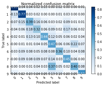
4.E.e.ii LBP Textural AdaBoost

pred = adaboost_tex.predict(textural_features_test)
draw_confusion_matrix(test_labels, pred)

Accuracy = 0.495
Confusion Matrix =
[[0.828 0.04  0.044 0.017 0.03  0.002 0.024 0.001 0.    0.014]
 [0.13  0.772 0.025 0.021 0.002 0.002 0.015 0.028 0.    0.004]
 [0.068 0.146 0.394 0.162 0.062 0.026 0.023 0.093 0.014 0.012]
 [0.04  0.056 0.176 0.318 0.062 0.09  0.016 0.168 0.058 0.017]
 [0.023 0.014 0.128 0.104 0.438 0.125 0.054 0.055 0.024 0.035]
 [0.001 0.012 0.014 0.036 0.052 0.475 0.062 0.056 0.22  0.072]
 [0.032 0.088 0.076 0.054 0.084 0.078 0.362 0.098 0.044 0.084]
 [0.    0.087 0.08  0.092 0.066 0.138 0.027 0.448 0.058 0.004]
 [0.    0.003 0.01  0.04  0.029 0.373 0.051 0.019 0.396 0.078]
 [0.062 0.018 0.031 0.044 0.049 0.126 0.096 0.004 0.053 0.518]]

<matplotlib.axes._subplots.AxesSubplot at 0x7fd459f914a8>

4.E.e.iii HOG Textural AdaBoost

pred = adaboost_tex_hog.predict(textural_features_hog_test)
draw_confusion_matrix(test_labels, pred)

Accuracy = 0.84905
Confusion Matrix =
[[0.947 0.025 0.    0.    0.006 0.019 0.    0.    0.    0.002]
 [0.09  0.889 0.004 0.    0.004 0.    0.007 0.    0.    0.004]
 [0.    0.008 0.902 0.062 0.006 0.    0.006 0.012 0.    0.003]
 [0.    0.    0.274 0.696 0.025 0.    0.002 0.    0.    0.   ]
 [0.002 0.008 0.158 0.384 0.431 0.01  0.002 0.    0.    0.004]
 [0.023 0.018 0.    0.    0.007 0.891 0.001 0.    0.058 0.   ]
 [0.    0.042 0.014 0.    0.01  0.002 0.858 0.02  0.    0.052]
 [0.001 0.004 0.012 0.003 0.    0.    0.009 0.97  0.    0.   ]
 [0.    0.011 0.    0.    0.003 0.008 0.003 0.    0.972 0.004]
 [0.002 0.014 0.006 0.    0.002 0.001 0.04  0.    0.    0.934]]

<matplotlib.axes._subplots.AxesSubplot at 0x7fef8c5600b8>

4.E.f RandomForest Evaluation

1. Geometric
2. Textural

4.E.f.i Geometrical Random Forest

pred = randomforest_geo.predict(geometrical_features_test)
draw_confusion_matrix(test_labels, pred)

Accuracy = 0.1001
Confusion Matrix =
[[0.122 0.1   0.114 0.089 0.08  0.1   0.094 0.093 0.1   0.108]
 [0.116 0.104 0.109 0.093 0.09  0.104 0.092 0.108 0.096 0.089]
 [0.128 0.116 0.11  0.088 0.089 0.098 0.086 0.088 0.106 0.092]
 [0.123 0.098 0.104 0.09  0.095 0.089 0.092 0.098 0.112 0.098]
 [0.114 0.102 0.113 0.092 0.086 0.088 0.116 0.086 0.094 0.107]
 [0.128 0.102 0.106 0.082 0.084 0.098 0.102 0.092 0.106 0.101]
 [0.112 0.104 0.109 0.098 0.08  0.094 0.1   0.092 0.107 0.104]
 [0.112 0.118 0.11  0.088 0.082 0.108 0.094 0.084 0.109 0.094]
 [0.125 0.098 0.108 0.083 0.076 0.102 0.11  0.099 0.102 0.097]
 [0.107 0.108 0.115 0.098 0.079 0.094 0.092 0.102 0.099 0.105]]

<matplotlib.axes._subplots.AxesSubplot at 0x7fd459c022e8>

4.E.f.ii HOG Textural Random Forest

pred = randomforest_tex_hog.predict(textural_features_hog_test)
draw_confusion_matrix(test_labels, pred)

Accuracy = 0.9796
Confusion Matrix =
[[0.974 0.02  0.    0.    0.    0.004 0.    0.001 0.    0.   ]
 [0.011 0.986 0.002 0.    0.    0.    0.    0.    0.    0.001]
 [0.    0.005 0.976 0.012 0.006 0.    0.    0.001 0.    0.002]
 [0.    0.    0.024 0.956 0.018 0.001 0.    0.    0.    0.   ]
 [0.    0.001 0.005 0.012 0.979 0.002 0.001 0.    0.    0.   ]
 [0.011 0.002 0.    0.    0.002 0.984 0.    0.    0.001 0.   ]
 [0.    0.002 0.    0.    0.    0.002 0.978 0.    0.    0.016]
 [0.    0.002 0.003 0.    0.    0.    0.002 0.992 0.    0.   ]
 [0.001 0.    0.    0.    0.    0.001 0.    0.    0.996 0.002]
 [0.002 0.006 0.    0.002 0.002 0.002 0.011 0.    0.    0.976]]

<matplotlib.axes._subplots.AxesSubplot at 0x7fef8c37ce48>